Curves of Constant Width
This page requires JavaScript for MathJax formatting and embedded GeoGebra files.
Introduction
Most 2D shapes you'll see in everyday life will have different widths depending on the direction in which you measure them. For example, a square with sides of length $s$ has a minimum width of $w = 1.0 × s$ when measured parallel to a side, and a maximum width of $w = \sqrt{2} × s ≈ 1.414 × s$ when measured along a diagonal (a precise definition of how to measure a shape's width is given in the Groundwork section below). The well-known exception to this variable-width property is the circle, which has the same width in all directions: its diameter.
The property of constant width is convenient in many different applications. One benefit of manhole covers being circular is that no matter how you turn them, they can't fall down the hole they cover. If you instead have a square opening and a square cover, you can easily drop the cover through the opening by rotating it a specific way in 3D space.
The constant-width property is also useful in coin-operated devices, where it allows for easy detection of what coins have been inserted in a mechanism by measuring their width alone. If you have a coin with non-constant width, that measurement would depend on the orientation of the coin when inserted, and a more complicated coin-identifying mechanism would be required.
Additionally, in the fields of engineering and manufacturing it is often necessary to construct things with circular profiles or cross-sections, and since we know that circles have a constant width, one of the most obvious ways to check whether or not something you've built is truly circular would be to see if its width is constant.
But is that enough? Are there any non-circular shapes that nevertheless have a constant width, independent of direction?
As you can probably guess from the title of this post, it turns out there are! In fact, there are multiple families of such Curves of Constant Width. While that complicates things for engineers, it opens up plenty of opportunities for interesting mathematics. Let's get to know a few of them!
Groundwork
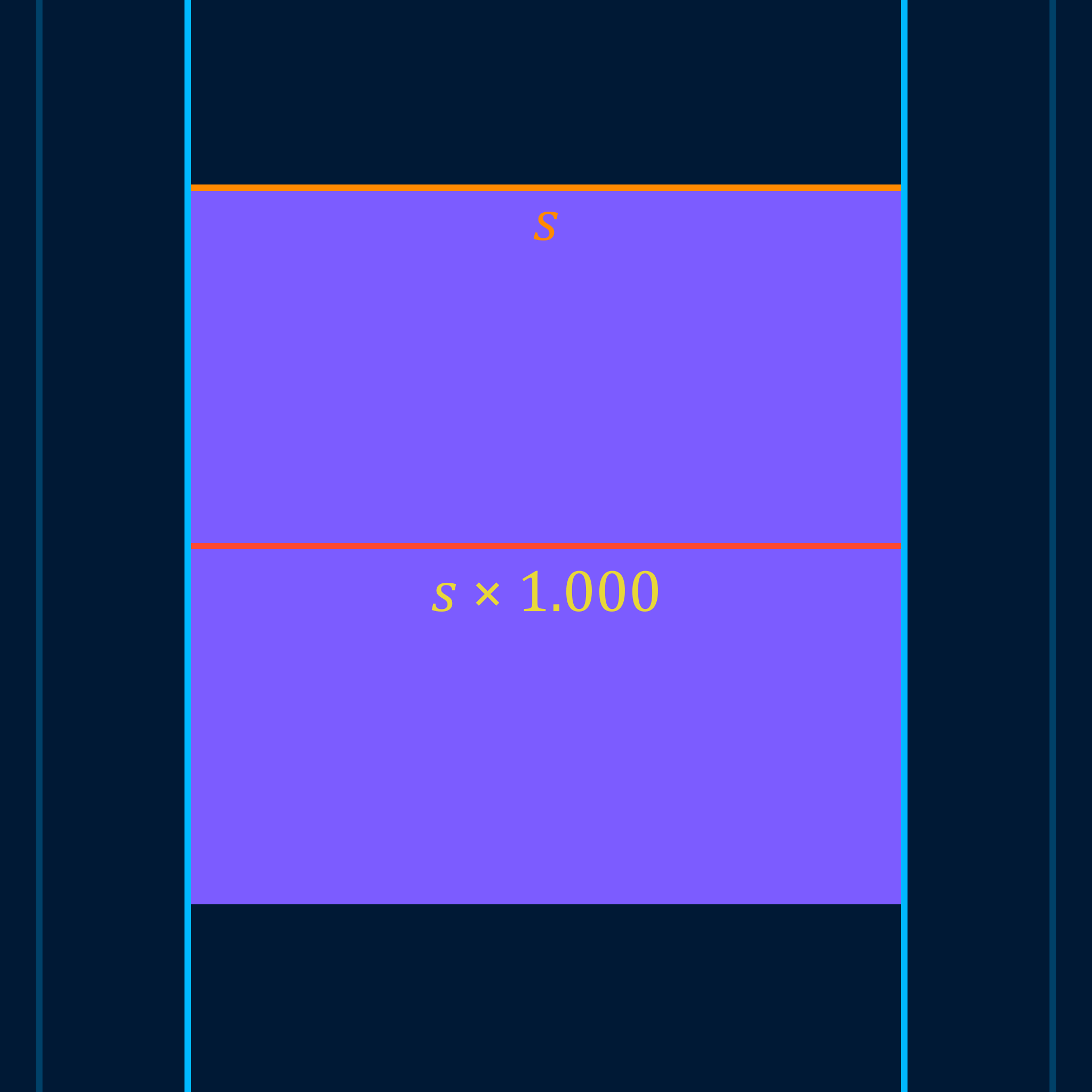
For the sake of clarity and rigor, in this post, a shape's width in a given direction is defined as "the distance between the two mutually-parallel supporting lines that are perpendicular to that direction", where a supporting line is "a line that touches the boundary of the shape at one or more points but does not cross the interior of the shape". In the animation below, the supporting lines are the moving vertical light-blue lines, and the measured width is shown as the red-and-yellow line between them.
Reuleaux Polygons
Aside from the circle, the simplest Curve of Constant Width (CoCW) to construct is the regular Reuleaux triangle, named after German mechanical engineer Franz Reuleaux. It can be created by replacing the three sides of an equilateral triangle with three circular arcs, with each arc having one vertex of the triangle as its center point and the other two vertices as its start and end points.

Any regular polygon (where all sides and angles are the same) with an odd number of sides can be converted into a regular Reuleaux polygon by replacing each straight edge with a circular arc centered on the opposite vertex. Of course, the greater the number of sides a regular polygon has, the closer it is to a circle, and the same fact is even more true for Reuleaux polygons due to their curved edges. As the polygon with the smallest possible number of sides, the regular Reuleaux triangle is the farthest away from being a circle and thus the most noteworthy of this family of shapes.
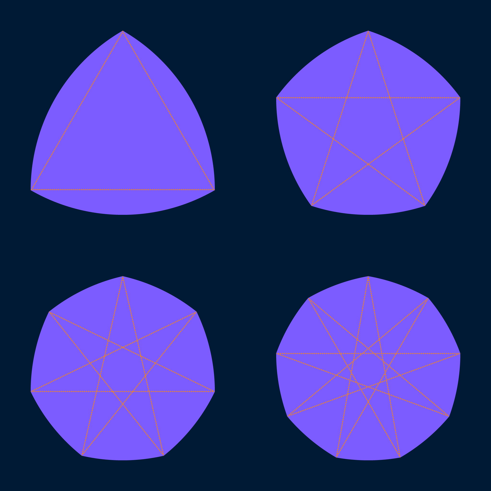
Some irregular polygons with an odd number of sides can also be converted into Reuleaux polygons. Such a polygon must be strictly convex (meaning all internal angles are less than 180 degrees and it has no self-intersections), and every vertex must be equidistant from its two opposite vertices. The construction of an irregular Reuleaux polygon is the same as that of a regular Reuleaux polygon, except that while all the circular arcs will still share the same radius, they will not all span the same angle.
There are no Reuleaux polygons with an even number of edge-arcs, because in a polygon with an even number of sides, each side is located opposite from another side instead of a vertex, which prevents the use of the Reuleaux construction process. However, there are other CoCWs with an even number of edge-arcs.
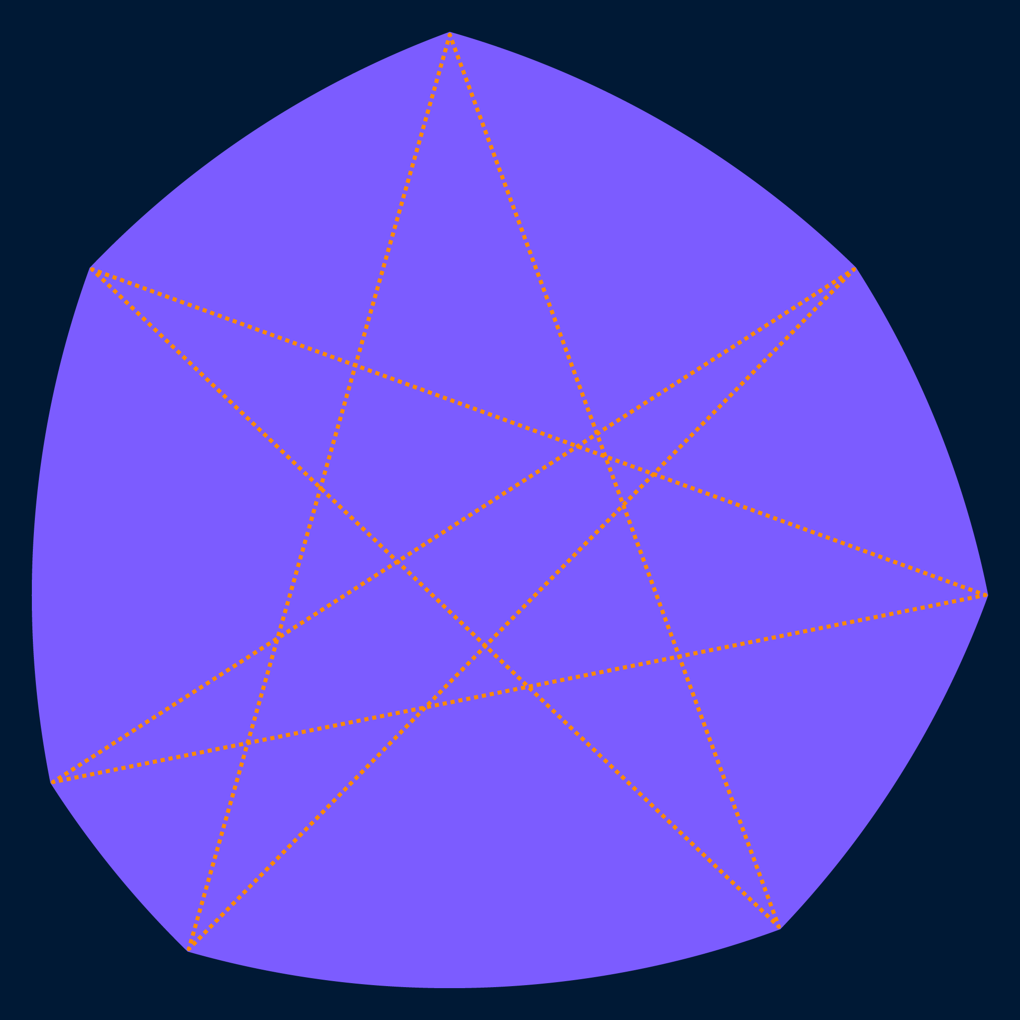
One of the simplest ways to construct a CoCW with an even number of edge-arcs is by taking any Reuleaux polygon, offsetting all of its edge-arcs outwards by the same amount (which increases their radii without changing their centerpoints or the angles they span), and connecting each of the gaps this creates with a new circular arc (shown in light-blue in the animation below) centered on the vertex at the center of the gap. This doubles the number of edge-arcs, making the number even. It also increases the number of non-zero arc-radii to two: the offset value, and the original radius plus the offset value.

Around the Corner: Geometric Continuity
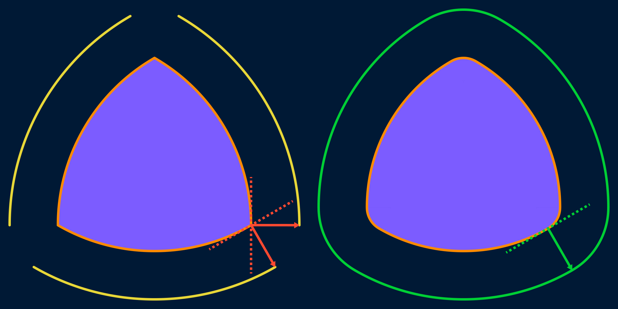
Notice that the expanded Reuleaux triangle in the above GIF becomes smoother — the starting shape has sharp corners, but the final shape does not. For a rigorous definition of "smoothness", we can look at the concept of geometric continuity. There are different levels or degrees of geometric continuity, denoted $G^n$ for non-negative integer $n.$ To qualify as $G^n$ continuous at a given point, a shape must satisfy the conditions for all levels from $0$ to $n$; put another way, a shape's degree of continuity at a point is "one less than the first level whose conditions it fails to meet". When looking at an entire shape, not just one point on the shape, the shape as a whole is considered to have the same degree of continuity as its least-continuous point(s).
Discontinuous
A shape with any gaps or openings in its boundary, sometimes called an "open" shape, has no geometric continuity.

G-Zero
Any "closed" shape, with no gaps in its boundary, has $G^0$ continuity. This is the case for all Reuleaux polygons, as well as their expansions.

G-One
The next level of continuity, $G^1$, requires that exactly one well-defined tangent line (a line that "just touches" a curve, with the same slope or angle as the curve at the point of contact) exists for all points on the shape; that is, the shape has no sharp corners, as a corner is a point with more than one tangent. Another way of defining this is to say that the path traced out by the end of the unit normal vector (a vector of constant length that is perpendicular to a curve at a given point) is continuous across the entire boundary of the shape. This is the case for expanded Reuleaux polygons, but not for Reuleaux polygons themselves.
In the animation below, the normal vectors are solid arrows and the tangents are dashed lines.
G-Two
$G^2$ continuity requires that the curvature is continuous along the entire boundary of the shape, where the "curvature" at a point on a curve is the inverse of the radius of the osculating circle at that point. An osculating circle, sometimes known as a kissing circle, is the circle that most closely fits a curve at a given point, i.e. is tangent to the curve at that point and at infinitesimally-close points on either side.
The more tightly a shape curves, the larger the curvature and the smaller the radius of the osculating circle. A straight line has zero curvature, equivalent to having an osculating circle of infinite radius, while a sharp corner has infinite curvature, equivalent to having an osculating circle of zero radius (if you accept that $\frac{1}{0} = ∞$ and $\frac{1}{∞} = 0$, which is not a given in all areas of mathematics but is valid enough in this specific case).
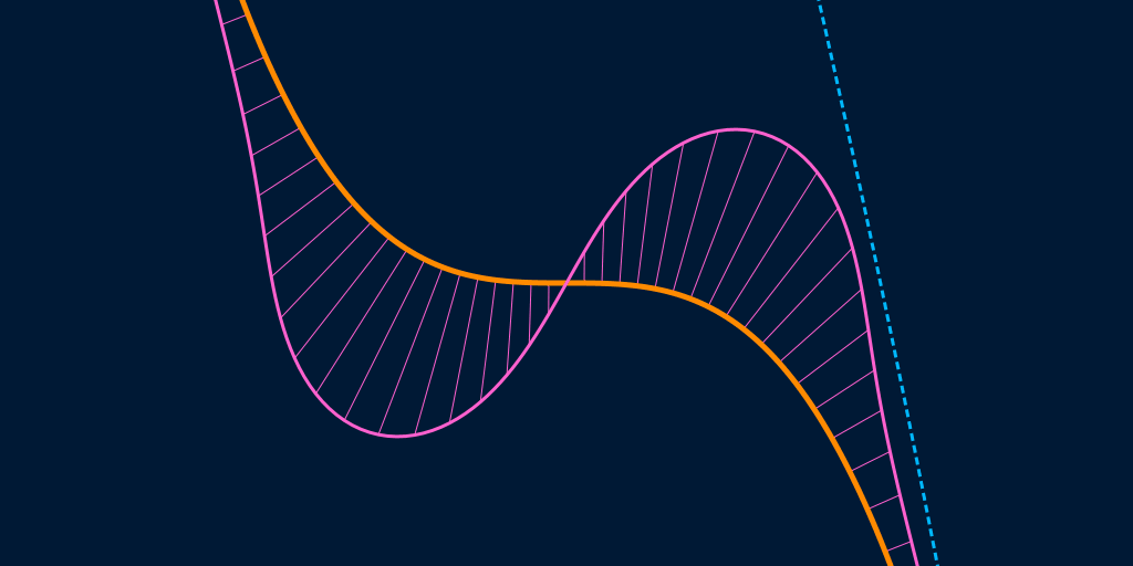
In the animation below, which shows the curvature and osculating circles of the graph of the open curve given by the equation $y = -x^3$, the curvature at the moving white point is shown in pink and the osculating circle at the white point is shown in light-blue. The thin pink lines connecting the main curve (orange) to the curvature plot (pink) are drawn to make it clear which part of the pink curve corresponds to a given part of the main curve; the curvature-curve-plus-connecting-lines combined structure is referred to as a curvature comb.
While each edge-arc of a Reuleaux polygon has the same radius and thus the same curvature, the sharp corners where neighboring edge-arcs join at the vertices have zero radius and infinite curvature, producing a discontinuity; so even if they hadn't already been disqualified, they would fail this test as well. And though expanded Reuleaux polygons do not have sharp corners, the radius of curvature is still discontinuous where the vertex-arcs with one radius are joined to the edge-arcs with a larger radius, so they also fail this test.
In the animation below, the osculating circle (and its radius) of the curve at the white point is shown in blue, while the curvature is shown in pink; once again, note that the bigger the radius, the smaller the curvature, and vice versa.

To create a Curve of constant Width with $G^2$ continuity, we need a different approach than stitching together multiple circular arcs. Luckily, there are other ways to construct constant-width curves.
Laying the Foundation: Support Functions
A 2D parametric curve is a shape whose Cartesian $(x, y)$ coordinates in 2D space are defined as functions of an additional parameter, for example time $t$ or angle $θ$ (theta), resulting in coordinates like $\bigl(x(t), y(t)\bigr)$ or $\bigl(x(θ), y(θ)\bigr).$
The support function $h(θ)$ of a closed convex 2D curve describes the signed distance between the origin (the point $(0, 0)$ on the Cartesian Plane) and the curve's supporting line in the direction given by rotating the positive $x$-axis clockwise by the angle $θ$ (recall the definition of supporting lines from the Groundwork section at the top of this post).
Note: I say signed distance because if the origin is not located inside the curve, the support function's output will be negative for some values of $θ$ (so the value may have either a plus or minus sign, hence the name). For simplicity's sake, in this post we'll assume the origin is contained by the curve and thus the support function is always positive.
For a CoCW of width $w$ and defined by an angular parameter $θ$ and support function $h(θ)$, the equation $h(θ) + h(θ + π) = w$ (where an angle of $π$ radians equals $180°$, so $θ + π$ points in the opposite direction from $θ$) must be true for all values of $θ$ by definition, as that is just another way of saying that the shape's width is constant in all directions.
The Cartesian coordinates of a curve can be defined in terms of the curve's support function $h(θ)$ and its derivative $h'(θ)$ as $$ x(θ) := \cos(θ) × h(θ) − \,\sin(θ) × h'(θ), \\ y(θ) := \,\sin(θ) × h(θ) + \cos(θ) × h'(θ). $$ Note: The COLON EQUALS sign specifies a definition, rather than an equivalence; the derivative of a function at a given input is the slope of the function at that input; and $\cos(θ)$ and $\sin(θ)$ are functions from trigonometry that are closely connected to rotations, circles, and periodic behavior.
To describe an arbitrary CoCW, let us establish the variables
- $w$ as the curve's width,
- $r$ as the curve's maximum radius of curvature, and
- $a$ as the curve's minimum radius of curvature,
with all three variables being non-negative real numbers and $0 ≤ a ≤ r ≤ w$ (where "$x ≤ y$" means "$x$ is less than or equal to $y$").
For any CoCW, the radius of curvature at any point, added to the radius of curvature at the directly opposite point, always sums up to the shape's overall width, so the above variables are related by the equation $w = r + a.$ (This fact may not be obvious at first, but consider: if the sum of opposing radii was less than the overall width at a given point, the shape would be curving more strongly inward than a circle of the same width on one or both sides, and thus the overall width would decrease as you moved to one side or the other of the initial measuring point; while if the sum of opposing radii was greater than the overall width, the shape would be curving less strongly inward than a circle of the same width on one or both sides, and thus the width would increase as you moved to one side or the other of the initial measuring point.)
We will also establish the variable $c$ as a measure of how far the shape is from a perfect circle, with $c = 0$ when $a = r$ (meaning the minimum and maximum radii are the same, thus the curvature is constant, thus the shape is a perfect circle) and with $c = 1$ when $a = 0$ (meaning the minimum radius is zero, which is the farthest it is possible to get from the maximum radius).
Using the width and circularity variables, we can construct definitions for the maximum and minimum radii as $r := \frac{w}{2} × (1 + c)$ and $a := \frac{w}{2} × (1 − c).$
Reuleaux Support
We can create Reuleaux polygons parametrically with the correct support function. We'll start with some definitions:
- The floor function returns the largest integer that is less than or equal to the input; for example, $\operatorname{floor}(3.14159) = 3$ and $\operatorname{floor}(−2.71828) = −3$.
- The modulo function (usually abbreviated to "mod") returns the remainder after dividing an input dividend $x$ by an input divisor $d$; put another way, it takes an input $x$ and adds or subtracts from it a divisor $d$ until the result is in the interval between zero (inclusive) and $d$ (exclusive). We will define it here as $$ \operatorname{mod}(x, d) := d × \left(\frac{x}{d} − \operatorname{floor}\left(\frac{x}{d}\right)\right). $$
- Finally, a piecewise function is a function whose input domain is divided into multiple pieces or cases based on conditions, written here in the form $$ \text{Function Name} := \begin{cases} \text{Case }1 & : \text{Condition }1 \\ \text{Case }2 & : \text{Condition }2 \\ ... \\ \text{Case }n & : \text{Condition }n \end{cases} $$ where for each input you start at the top of the list, check the input against each condition, and use the first case whose condition is true for that input. If you are familiar with programming, piecewise functions operate very much like IF–THEN–ELSE constructs (IF condition 1 is true THEN use statement 1, ELSE IF condition 2 is true THEN use statement 2, ELSE...).
Putting it all together, say we want a regular polygon with $n$ sides (where $n$ is an odd integer greater than or equal to $3$). If we define a helper function for conciseness $$ f(θ) := \operatorname{mod}\left(θ + \frac{π}{2 n}, \frac{2 π}{n}\right), $$ and give the support function the piecewise definition $$ h(θ) := \begin{cases} \frac{r − a}{2} × \sec\left(\frac{π}{2 n}\right) × \cos\left(f(θ) − 1 × \frac{π}{2 n}\right) + a & : 0 × \frac{π}{n} ≤ f(θ) < 1 × \frac{π}{n} \\ \frac{a − r}{2} × \sec\left(\frac{π}{2 n}\right) × \cos\left(f(θ) − 3 × \frac{π}{2 n}\right) + r & : 1 × \frac{π}{n} ≤ f(θ) < 2 × \frac{π}{n} \end{cases} $$ or, equivalently (by replacing $r$ and $a$ with their definitions from above and simplifying), $$ h(θ) := \frac{w}{2} × \begin{cases} 1 + c × \Bigl(\sec\left(\frac{π}{2 n}\right) × \cos\left(f(θ) − 1 × \frac{π}{2 n}\right) − 1\Bigr) & : 0 × \frac{π}{n} ≤ f(θ) < 1 × \frac{π}{n} \\ 1 − c × \Bigl(\sec\left(\frac{π}{2 n}\right) × \cos\left(f(θ) − 3 × \frac{π}{2 n}\right) − 1\Bigr) & : 1 × \frac{π}{n} ≤ f(θ) < 2 × \frac{π}{n} \end{cases} $$ (where $\sec(θ)$ is another function from trigonometry) the resulting curve will be a regular Reuleaux polygon with $n$ sides and initial width $r − a$, expanded to the width $w = r + a.$ If $a = 0$, there is no expansion, and the resulting curve is simply a regular $n$-sided Reuleaux polygon of width $w = r.$
Below is an interactive plot of the Reuleaux curve, with the following controls:
- At the top of the plot, you can adjust the white sliders to change the number of sides $n$, the width $w$, and the circularity $c$; calculated values for $r$ and $a$ are shown below the $c$ slider. Changing the value for $w$ rescales the entire plot in the curve-view and thus has little visual effect there besides the $r$ and $a$ values, but its effect is more noticeable in the function-view.
- In the lower left of the plot, a button allows you to switch between viewing the Reuleaux curve (curve-view) and viewing the functions that go into generating the curve (function-view). As already mentioned, the $w$ slider's effect is more visible in the function-view.
- At the bottom of the plot, in curve-view checkboxes allow you to show or hide the vertices and line segments of the traditional construction of an equivalent Reuleaux polygon, as well as the curvature comb, supporting lines, and osculating circles of the plotted curve, while in function-view the checkboxes allow you to show or hide specific functions.
- On the left side of the plot in curve-view, when the supporting lines and/or osculating circles are visible a green slider appears that allows you to change the angle of measurement $θ$ and the green point on the curve, while the yellow point is always $180°$ around the curve from the green point. The red point shows the center of curvature for a given value of $θ$; notice how it jumps around as you change the value of $θ$, while the measuring line rotates around it.

Smooth Support
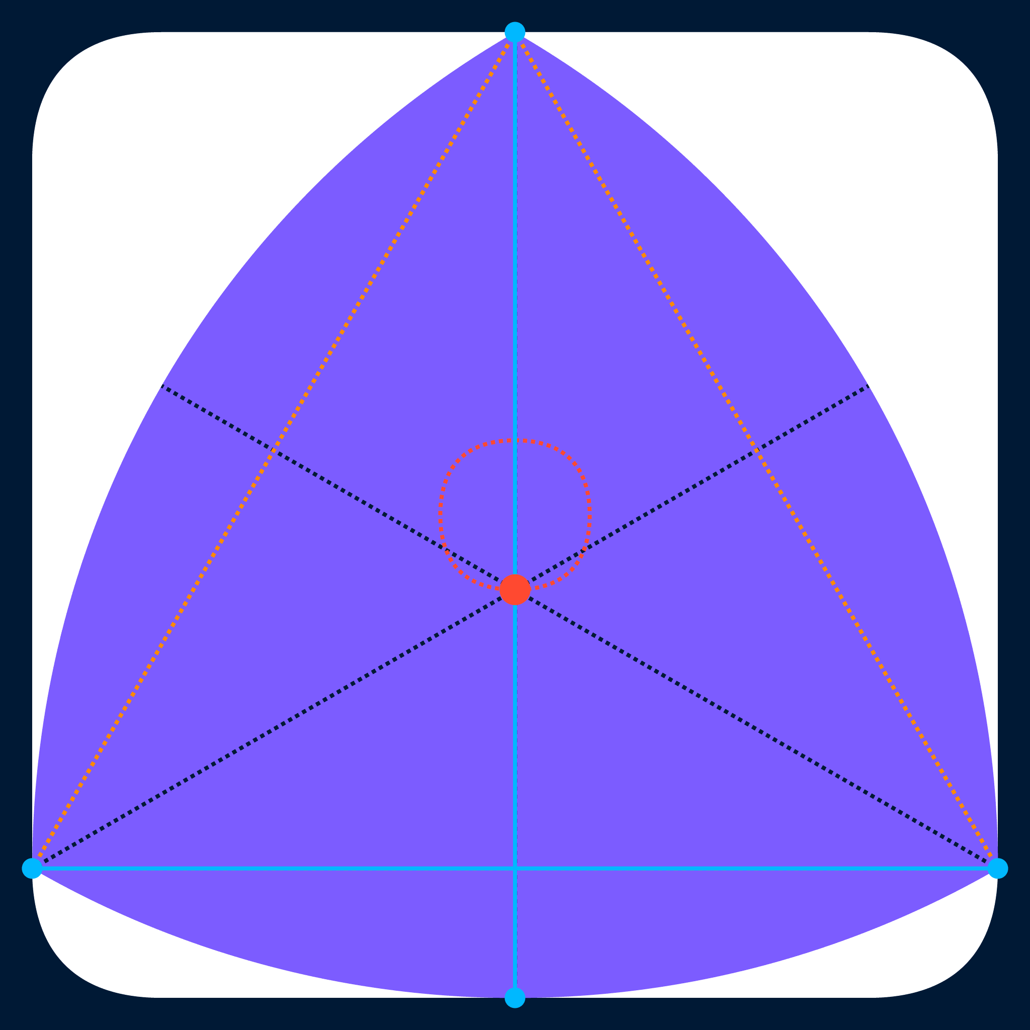
Of course, the reason for introducing the concept of support functions in this post was to provide a way to generate smoother shapes, not just an alternate way to generate the same shapes we'd already seen. If we swap out the piecewise support function definition above for the continuous support function $$ p(θ) := \frac{w}{2} × \left(1 + c × \frac{\cos(n × θ)}{n^2 − 1}\right) $$ the resulting curve will be a CoCW of width $w$ with $n$-fold rotational symmetry (approximating an $n$-sided regular polygon), maximum radii $r = \frac{w}{2} × (1 + c)$, and minimum radii $a = \frac{w}{2} × (1 − c).$ As long as $c$ is both non-negative and less than $1$, the shape will be $G^2$ continuous. In the special case where $c = 1$, the minimum radius of curvature reaches zero, creating sharp corners that drop the continuity back down to $G^1.$
Below is an interactive plot of the smooth curve. The setup is the same as that of the interactive Reuleaux curve in the previous section, except that the Reuleaux construction elements have been replaced by the curve's evolute, which is the curve traced out by the center of curvature (the red point again) as you move around the main curve (in the Reuleaux version, the evolute is made up of isolated points instead of a contiguous curve).

Properties of 2D Curves of Constant Width
All 2D CoCWs have a perimeter (the total length of their boundary curve(s)) of $π × w.$ This is known as Barbier's theorem after Joseph-Émile Barbier, the French mathematician who published it in 1860. A circle's circumference of $2π$ times its radius is just a special case of this fact, as a circle's radius is half its width.
However, CoCWs of the same width can have different areas. For a given width or perimeter, the CoCW with the greatest possible area is a circle, at $A = π × \left(\frac{w}{2}\right)^2.$ The CoCW with the smallest possible area is a non-expanded regular Reuleaux triangle, at $$ \begin{align} A &= π × \left(\frac{w}{2}\right)^2 × \left(2 − \frac{2 \sqrt{3}}{π}\right), \\ &= \frac{w^2}{2} × \left(π − \sqrt{3}\right), \end{align} $$ or approximately 89.73% of the area of a circle with the same width; this is known as the Blaschke–Lebesgue theorem after Austrian mathematician Wilhelm Blaschke and French mathematician Henri Lebesgue, who independently published it in 1915 and 1914, respectively.
The area of a regular expanded (or unexpanded for $c = 1$) $n$-sided Reuleaux polygon of width $w$ is $$ A = π × \left(\frac{w}{2}\right)^2 × \left(1 + c^2 × \left(1 − \frac{2 n}{π} × \tan\left(\frac{π}{2 n}\right)\right)\right). $$ This equation can be derived by adding up the areas of the $n$ circular sectors (pie-wedge shapes) that make up the edge-curves of the Reuleaux polygon, subtracting enough copies of the area of the inner straight-sided polygon to eliminate the overlaps, and (for expanded Reuleaux polygons) adding the areas of the $n$ circular sectors that make up the vertex-curves.
Using calculus, the area of a general CoCW can be written in terms of the curve's support function and its derivative with the integral $$ A = \frac{1}{2} × \int_{0}^{2π}{\big(h(θ)^2 − h'(θ)^2\big) dθ}. $$ For Reuleaux polygons, that evaluates to the equation in the previous paragraph. For the smooth support function shown in the previous section, that evaluates to $$ A = π × \left(\frac{w}{2}\right)^2 × \left(1 + c^2 × \left(\frac{1}{2 × \left(1 − n^2\right)}\right)\right). $$ The minimum area for that curve, where a $n = 3$ and $c = 1$, is $A = π × \left(\frac{w}{2}\right)^2 × \frac{15}{16}$, or 93.75% of the area of a circle with the same width (approximately 4.02 percentage points larger than the equivalent Reuleaux triangle).
Square Up
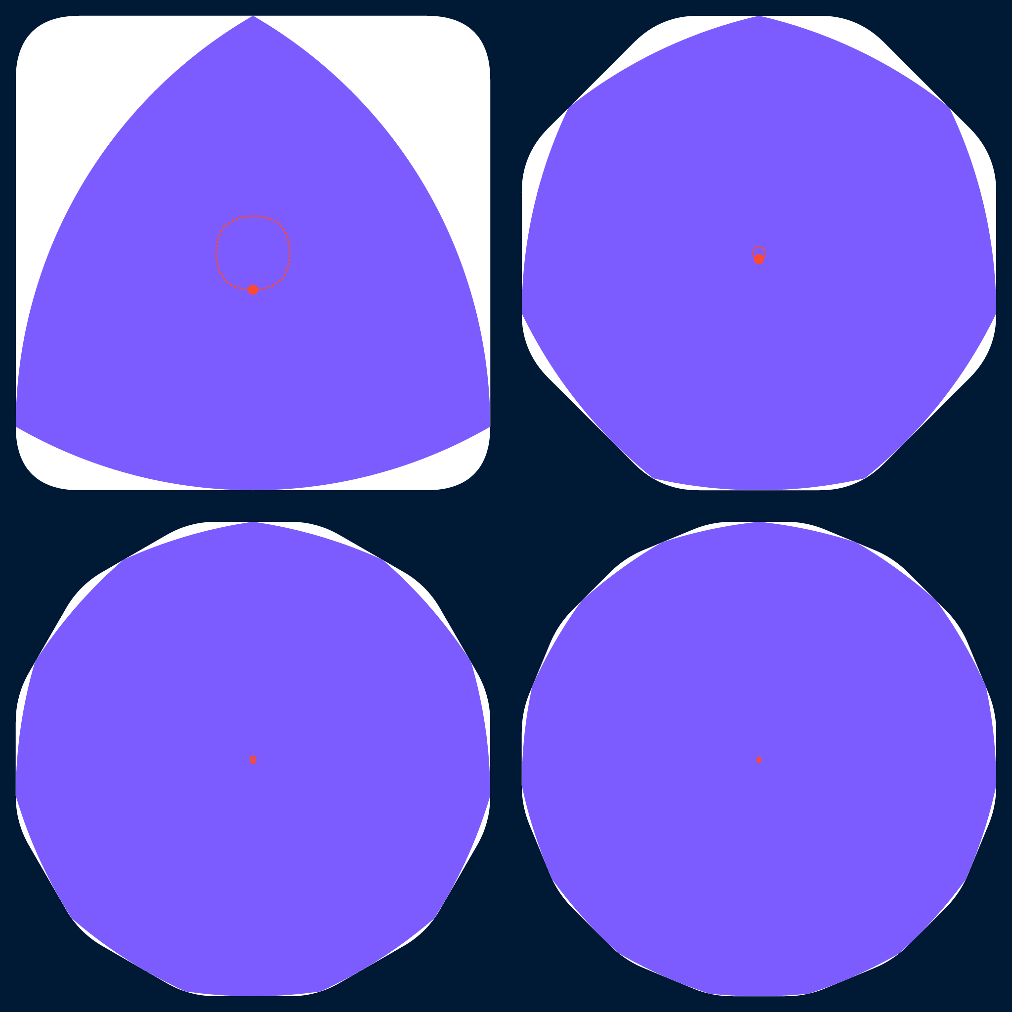
Another property of CoCWs is that they can all rotate inside squares with side lengths equal to the CoCW's width, while at all times remaining in contact with all four sides at exactly one point each.
The CoCW will not touch all points of the square during its rotation, however; the traced out shape may be a different polygon nested inside the square, and it will have rounded corners. The portion of the square's area which is covered during a full rotation depends on the specific CoCW being used, particularly its number of sides $n$ and minimum radius of curvature $a$; the greater the values of $n$ or $a$, the smaller the covered area will be. And this isn't limited to just squares: many CoCWs will rotate within rhombi, hexagons, and various other polygons while remaining in contact with every side.
Aside from a circle, CoCWs rotating within a square or other polygon cannot rotate on a fixed "axle" point, as their geometric centers (a.k.a. centroids) are not their centers of curvature. The path traced by the centroid across a full rotation will vary depending on both the CoCW and the bounding polygon.
Of the CoCWs that have been discussed in this post so far, the one that covers the maximum possible area across a full rotation is the (non-expanded) regular Reuleaux triangle. In the GIF below, the red dot shows the centroid of the rotating Reuleaux triangle, the red dashed line shows the path the centroid traces out as the shape rotates, the blue dots show the contact points between the triangle and the bounding square, and the blue lines highlight the fact that opposing contact points are always directly across from one another.
In particular, as they rotate inside a square, regular Reuleaux polygons with $n$ sides (and their expanded versions, as well as the analogous smooth CoCWs introduced in this post) will trace out round-cornered regular polygons with widths (measured perpendicular to their sides) equal to the width of the CoCW and with $4 × \operatorname{round}\left(\frac{n}{4}\right)$ sides (effectively, the closest multiple of four to $n$):
- triangles (3) and pentagons (5) trace out squares (4 sides),
- heptagons (7) and nonagons (9) trace out octagons (8 sides),
- hendecagons (11) and tridecagons (13) trace out dodecagons (12 sides),
and so on, always touching each side of the traced-out shape (and of the overall square) at exactly one point. As $n$ and/or $a$ increase, the area of the CoCW and the area of the shape it rotates within become closer and closer together as both shapes approach a circle.
If a CoCW is rotating within a square centered on the origin and is defined using a support function $h(θ)$, that function can be used to give the position of (and the path traced out by) the shape's centroid at rotation-angle $α$ as $$ x(α) := \frac{w}{2} − h\left(\frac{0}{2} − α\right), \\ y(α) := \frac{w}{2} − h\left(\frac{π}{2} − α\right). $$
An interesting consequence of the rotating-within-a-polygon property is that CoCWs can be used to drill holes in the shape of the polygons they rotate within. The drilled hole will have the same rounded corners as seen in the animations above, and the fact that the axel cannot be fixed in one spot makes the construction and mounting of a CoCW drill-bit non-trivial, so this is more of a party-trick than a practical application... but it's still pretty cool.
Conclusion
Unfortunately for engineers who want to build perfectly circular things, as you have now seen, there are many ways for a non-circular shape to have a constant width, and it may be hard to tell by eye how non-circular such a shape actually is. And there are several more ways to construct Curves of Constant Width that were not covered in this post. While this has not been an exhaustive list of every type of Curve of Constant Width there is, hopefully you have a new appreciation for the wonderful world of weird shapes!
Teaser: Journey Into Another Dimension
The property of constant width can be extended into three dimensions with Solids of Constant Width (SoCWs). But that's a big enough topic that it will have to wait for its own post.